In the complex world of systems engineering and real-time software development, understanding when something happens is often just as critical as understanding what happens. While traditional UML diagrams excel at modeling structure, behavior, and interaction sequences, they often fall short when precise timing constraints, duration requirements, and temporal synchronization become central to system correctness.
Enter the UML Timing Diagram—a specialized interaction diagram purpose-built for modeling time-dependent behaviors. Whether you're designing safety-critical automotive systems, industrial automation controllers, network protocols, or embedded firmware, Timing Diagrams provide the visual precision needed to specify, validate, and communicate temporal requirements with engineering rigor.
This comprehensive guide walks you through the fundamentals of UML Timing Diagrams using a realistic security gate scenario, explores advanced concepts through diverse engineering examples, and provides practical guidelines for creating clear, maintainable diagrams. By the end, you'll have the knowledge to apply Timing Diagrams confidently in your own real-time system designs.
Timing diagrams are fundamental when the sequence of events is less important than precise timing or duration of states.
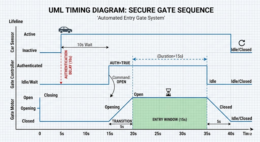
Imagine we are designing a security gate for a corporate parking lot. The requirements specify a strict sequence of hardware interactions based on timing constraints to ensure safety and security.
System Requirements:
Idle State: The system waits. The Gate Sensor reads 0 (No car), and the Physical Gate is CLOSED.
Detection: When a car arrives, the Gate Sensor detects it (changes from 0 to 1). This is Time $T=0$.
Authentication Delay: The main controller (Gate Controller) requires exactly 10 seconds (10s) to authenticate the vehicle RFID tag after detection. The Gate cannot open before this.
Opening Sequence: Once authenticated (at $T=10s$), the Gate Controller sends an 'OPEN' command to the Physical Gate.
Physical Response: The motor-driven Physical Gate takes exactly 5 seconds to transition from CLOSED to fully OPEN.
Entry Duration: The gate must remain open for exactly 15 seconds to allow the vehicle to pass through.
Closing Sequence: After the 15s entry window, the Gate Controller sends the 'CLOSE' command to the Physical Gate.
Physical Response: The motor takes 5 seconds to transition from fully OPEN to fully CLOSED.
Reset: During closing, the car must have cleared the Sensor. The system returns to Idle.
The Challenge:
Create a UML Timing Diagram that visually models this interaction between the Gate Sensor, Gate Controller, and Physical Gate Lifelines over a 40-second operational cycle.
The image below is the generated solution for the "Secure Automated Entry Gate" problem.
When analyzing the diagram above, note the foundational concepts defined in UML 2.5:
A Lifeline represents an individual participant in the interaction (e.g., Gate Controller). Unlike Sequence diagrams, which show vertical lifelines, Timing diagrams lay lifelines horizontally, stacked vertically.
The main horizontal axis shows how a Lifeline's state changes over time.
Discrete State: Used when objects have clear, distinct conditions (e.g., Idle, Opening, Closed). The line jumps orthogonally. This is used in the Secure Automated Entry Gate diagram.
Continuous State (or Value Lifeline): Used for non-discrete values (e.g., Temperature, Speed). The line creates curves or gradients.
The primary dimension is Time, flowing strictly from left to right. It is often calibrated with specific tick marks (e.g., 0s, 5s, 10s).
This constraint specifies that the Lifeline must remain in a specific state for a defined relative time (not an absolute timestamp).
In the Secure Automated Entry Gate diagram: {Duration=15s} is applied to the 'Open' state of the Gate Motor.
A constraint that specifies that an event must happen at a precise absolute time.
Timing diagrams show when a message is sent. Messages are usually horizontal arrows connecting two different lifelines, showing cause-and-effect.
These diagrams illustrate how the concept is applied across different engineering domains.
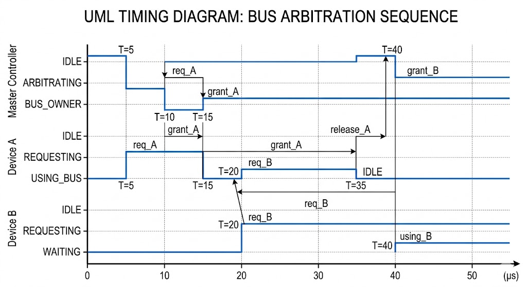
This example shows how multiple devices contend for control of a shared communication data bus. Timing is everything.
The Scenario:
A Controller and two Devices (A and B) use a shared Data Bus. A strict sequence of REQUEST, GRANT, and RELEASE signals (often requiring nanosecond precision) prevents data collision.
Key Insight: Notice how Device B must wait precisely until Device A releases the Bus (GRANT signal falls).
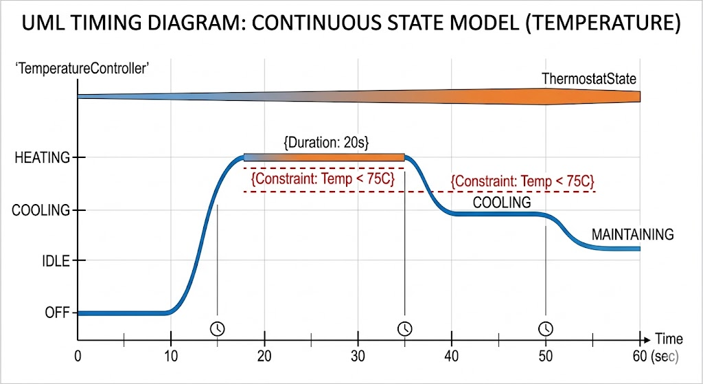
Many physical systems do not jump instantly between states. This diagram demonstrates how UML models analog or continuous physical values, like temperature or speed.
The Scenario:
A smart thermostat manages an industrial boiler. The system is safe only when the water temperature is within a target window.
Key Insight: This diagram uses a Continuous State Lifeline (the curvy line) for 'Water Temp'. It includes shaded zones showing when the state is within the required Duration Constraint. Notice how the linear 'Boiler State' (digital ON/OFF) must be carefully synchronized with the analog temperature curve.
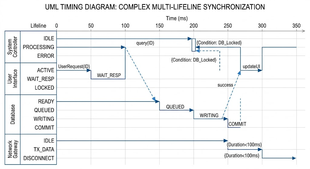
This example models a production line, showing how a primary process must synchronize with secondary, asynchronous events (like human interaction or resource availability).
The Scenario:
An Automated Assembly robot is building a product. It interacts with an Inventory system and a specialized Tooling station. The robot cannot proceed to 'Assembling' until both the specialized Tool is ready AND the Inventory has been reserved.
Key Insight: This diagram emphasizes complex synchronization. Two independent message arrows (from Inventory at $T=15$ and Tooling at $T=20$) are required to trigger the Robot's transition to 'Assembling' (at $T=25$). The diagram visualizes the dependency delays.
When creating or reading UML Timing Diagrams, apply these rules for clarity and technical accuracy.
Strict Left-to-Right Time: The horizontal dimension is time. It must be linear and monotonic. It cannot reverse.
Stacking Order: Lifelines that interact frequently or have causal relationships should be stacked adjacent to each other. This keeps message arrows short and the diagram clean (see the Secure Automated Entry Gate diagram and the Bus Arbitration diagram).
Use Constraints, Not Just Curves: The actual value of the timing diagram is the formal Constraint (e.g., {Duration < 50ms}). Don't rely solely on the visual length of the line; explicitly state the requirement.
Define States Locally: Define the possible states on the vertical axis (y-axis) for each Lifeline separately.
Optimize Messages:
Synchronous Messages (solid line, filled head): Use when the sender waits for a specific time event in the receiver before continuing.
Asynchronous Messages (dashed line, open head): Use when the message is a trigger and the sender continues its own timeline immediately (often used in distributed hardware).
Combine State Types Wisely: You can mix discrete (orthogonal) and continuous (curved) lifelines in the same diagram. (See the Industrial Thermostat diagram, combining the boiler's ON/OFF with the continuous temperature curve).
Identify Critical Causal Links: Timing diagrams excel at visualizing causation. Use strong vertical or curved arrows to show that Event A on Lifeline 1 causes Event B on Lifeline 2.
Don't Model Simple Logic: If your system is purely defined by sequence (e.g., A always follows B), use a Sequence Diagram. If you only need to show a simple change in state, use a State Machine Diagram. Only use Timing Diagrams when duration or precise timestamps are requirements.
Avoid Crowding Lifelines: If you have more than 5 or 6 lifelines, your timing diagram will likely become unreadable. Consider breaking the interaction into smaller sub-diagrams, or using State Machines with time-based triggers.
Clarity in Jumps: When a Lifeline changes state instantly, the vertical line must be perfectly orthogonal (90 degrees). Use ramps only if you are deliberately modeling a continuous transition (like the 'Opening' state in the Secure Automated Entry Gate diagram).
Visual Paradigm provides comprehensive support for UML Timing Diagrams, a type of interaction diagram used to visualize the behavior of objects over a specific period of time. It is particularly useful for modeling real-time and distributed systems where timing constraints are critical.
Visual Paradigm supports several modeling styles and components required for professional-grade specifications:
Notation Styles: The tool supports both Concise (state timeline) and Robust (general value lifeline) notation styles.
Visual Structure: Unlike sequence diagrams, timing diagrams in Visual Paradigm reverse the axes—time increases from left to right, and lifelines are arranged in separate vertical compartments.
Constraint Management: Users can easily add duration constraints, state transitions, and time messages between different lifelines.
Group Editing: A "blue line" feature allows you to move groups of time instances at the same state/condition simultaneously, simplifying major timeline adjustments.
You can follow these steps within the Visual Paradigm desktop application:
Start New Diagram: Select Diagram > New from the application toolbar.
Select Type: Choose Timing Diagram from the list of available UML diagrams and click Next.
Configure: Enter a name and description, then click OK to open the drawing canvas.
Add Frames: Use the Timing Frame tool on the diagram toolbar to place a frame, which usually starts with the sd keyword.
Define Timeline: Double-click on lifeline names, states, or time units to rename them and build out the specific temporal behavior of your system.
For those looking for a lightweight option, the Visual Paradigm Community Edition is a free UML modeler that supports all UML diagram types, including timing diagrams.
Would you like to see an example of how to model a specific real-time scenario, such as a traffic light system or a network protocol, using these tools?
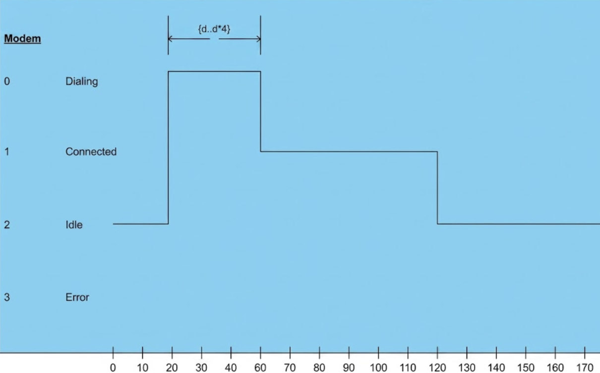
The diagram tracks the state changes of a Modem over a timeline of 190 units. The modem transitions between three specific functional states: Idle, Dialing, and Connected, while an Error state is defined but not utilized in this specific sequence.
The sequence of events unfolds as follows:
Initial State (0 to 20 units): The modem starts in the Idle state.
Transition to Dialing (at 20 units): The modem transitions vertically to the Dialing state.
Dialing Duration and Constraint: The modem remains in the Dialing state from time 20 to time 60. This period is marked with a timing constraint of {d..d*4}, indicating the allowable duration for this specific action.
Transition to Connected (at 60 units): Once the dialing process is complete, the modem drops to the Connected state.
Connection Maintenance (60 to 120 units): The modem maintains an active connection for 60 units of time.
Return to Idle (at 120 units): The modem transitions back down to the Idle state, where it remains for the rest of the observed timeline (up to 190 units).
State Hierarchy: The states are listed on the y-axis, with Dialing at the highest tier (0), Connected in the middle (1), and Idle near the bottom (2).
Time Scale: The x-axis provides a ruler with increments of 10 units, allowing for precise measurement of state durations.
UML Timing Diagrams are an indispensable tool for engineers working on systems where time is not just a factor—it's a requirement. From automotive safety systems and industrial automation to network protocols and embedded devices, the ability to precisely model durations, deadlines, and synchronization points can mean the difference between a robust design and a critical failure.
This guide has equipped you with:
A clear understanding of when to choose Timing Diagrams over other UML interaction diagrams
Practical experience modeling a real-world security gate system with strict temporal constraints
Exposure to advanced patterns including continuous state modeling and multi-lifeline synchronization
Actionable guidelines to create clear, maintainable, and technically accurate diagrams
Remember: Timing Diagrams shine when precision matters. Use them to document requirements, validate designs with stakeholders, and communicate temporal logic to development teams. With tools like Visual Paradigm supporting the full UML 2.5 specification, creating professional-grade Timing Diagrams has never been more accessible.
As real-time and safety-critical systems continue to proliferate across industries—from autonomous vehicles to medical devices—the skill of modeling time explicitly will only grow in value. Master Timing Diagrams today, and you'll be better prepared to engineer the reliable, predictable systems of tomorrow.